People wanting to learn about the "guts" of APE or how to program automated polarization measurement code
People seeking the answer to "life, the universe and everything"
2. APE General Layout
GUI The APE program "lives" in two windows. First, in the shell that pops up after choosing ape from the "SLS Launcher".
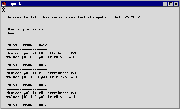
This shell will display information about APE operation and user interaction. This info will be pretty boring, but can be used for debugging purposes or as a "log book" of a measurement run (save contents before quitting ape or else they will be lost). Most users will not be interested much in this window. If you do not want to see the shell minimize it, but do NOT close the shell window - it will kill APE and this is definitely not what you want to do (see further below).
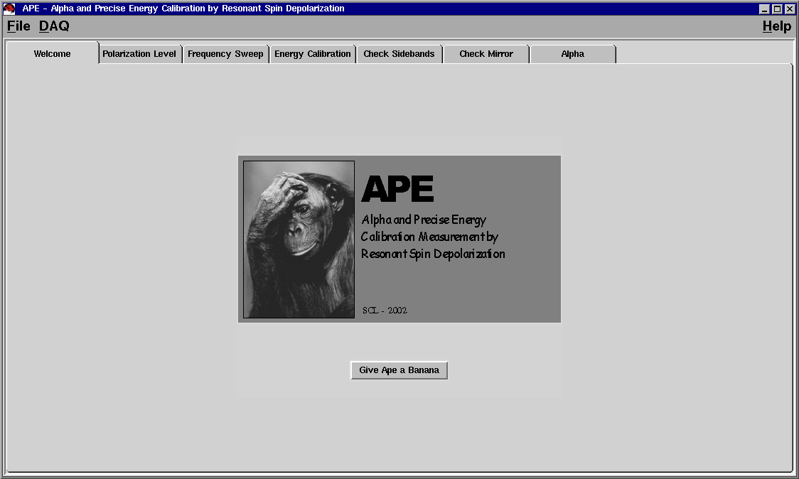
The second window is APE's GUI and will be the place where users interact with the program. It shows up shortly after starting the program.
This window consists of two parts. The upper is a menu bar which contains the menus "File", "DAQ", and "HELP". The menu "File" contains entries to take screen shots of APE's GUI window and a quit command. Please always exit APE through this quit command; do not use window manager close/kill commands or a ctrl-c in the shell! APE runs all sorts off background processes which are only terminated properly when using the quit button. If you exit APE by other means these processes could continue running, putting a great load on the CPU and eventually fill up the HD or RAM. In case APE is not properly closed a lock file will be left behind. In an attempt to re-launch APE or to run a second copy of APE simultaneously the lock file will be detected and APE will not start. Before you remove such a lock file manually, make sure that no APE process or APE background process is running anymore. Simultaneous operation of multiple APE processes will lead to ruined data files, uncertain experimental conditions and possibly a screwed up machine! The "DAQ" menu contains status and control of the data acquisition as well as a command to save acquired data to a data file. Finally, the "Help" menu leads to this manual which you already have noticed since you are reading these lines.
The lower part of the window is a tab interface which allows the user to perform the different experimental runs and see data as well as start, stop and see fits.
Color Code APE uses a color code to help the user understand the meaning of GUI elements. Normal text/numbers are black as well as button text. Red is used to highlight important results or to show critical read-back values.
White backgrounds show read-back values whereas grey backgrounds show that a field is for user-input of set-values.
3. Screen Grabbing
In the "File" menu a user can select two screen grab entries. Both of them do the same thing and work the same way; the only difference is that one command grabs to a gif file (good for web publication) whereas the other grabs to a ps file (good for printing). When the user selects the screen grab entry he/she is presented with a dialog to select the name and location for the grab file. Shortly after this selection is confirmed by the user, two beeps tell the user that the screen is being dumped now. The grab will be written to the file defined by the user.
4. Data Acquisition
Data acquisition related stuff is in the second menu. The first two entries are radio buttons for turning on and off the data acquisition. Data acquisition starts when the "On" radio button is selected. The data will be used by APE internally. Once the data acquisition is turned off the user is asked if he/she wants to save the acquired data to an APE data file (the location can be selected by the user). Even if you do not choose to have APE save to a DAQ file, the acquired data will be present for APE to analyze, but it will be purged as soon as the next data acquisition is started.At any time (even during data acquisition) the user can save the acquired data to an APE data file by selecting the "Save DAQ File..." entry. Again the save location can be chosen by the user. If the data acquisition is off and a user chooses the "Save DAQ File..." entry the last acquired data is saved; this could even be the data of a run performed when APE was last used! Vise-versa is also possible - you could copy an old DAQ file to APE's tmp directory and start APE to do some off-line analysis of the old data. As long as the user doesn't turn the data acquisition on, the existing DAQ file will not be purged.
5. Polarization Level
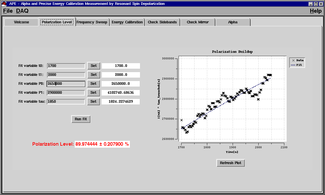
The second tab in APE's GUI window leads to the polarization level measurements.
On the left side fit parameters can be set and read back. Also, the fit can be triggered and as a result the polarization level is displayed. The right side shows a plot of I*tau vs. time as well as a polarization build-up fit. The plot will not constantly refresh, use the button for this.
Procedure
Once a build-up process has begun the initial fit values have to be set. t0 and t1 mark the beginning and end (on the time scale) of the fit interval, P0 and P1 are the bottom and top level of the data with respect to the y axis (P0 is the product of I*tau at the point t0 and likewise for P1) and tau is the time constant for the exponential buildup process (a good start-up value is 1700 s). Once these values are set, press the "Run Fit" button; this will start the fitting procedure. As a result the polarization level reading is updated as well as the optimized fit values P1 and tau. The plot on the right side will now also show the updated fit curve.
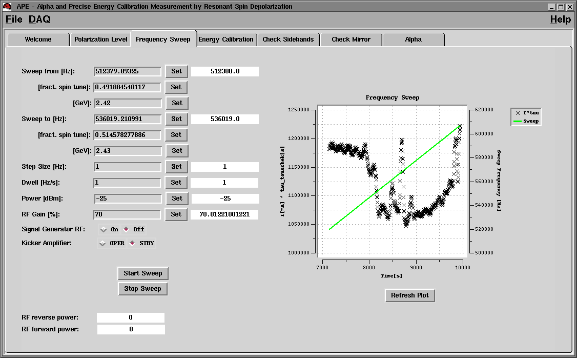
6. Frequency Sweep
The third tab in APE's GUI window leads to the frequency sweep.
The left side shows settings for the sweep, two buttons to start and stop a sweep and read-backs for the forward and reverse power of the kicker amplifier. The right side shows a plot of current*lifetime vs. time as well as the sweep frequency vs. time.
Procedure
Set the sweep interval in Hz (alternatively this interval can be set in units of the fractional spin tune or in corresponding beam energy in GeV), the step size (by how many Hz to increase the sweep frequency per step) and the dwell (how many seconds to stay at one sweep step). Next, set the power of the signal generator output in dBm (normally: -30 dBm < power < -5dBm) and the gain of the amplifier in percent. Finally set the signal generator's RF to on or off and the kicker amplifier to operational (OPER) or stand-by (STBY). Warning: If you set the signal generator RF to "On", the kicker amplifier to "OPER" and start the sweep you will apply power to the kicker magnet and perturb the beam! Only do this if you really know what you are doing and are ready to do the experiment. For debugging or testing purposes set the signal generator RF to "Off" or the amplifier to "STBY". You can now start the sweep by pressing the "Start Sweep" button. While running a sweep the forward and reverse power read-back should show what actual power is applied by the amplifier to the kicker magnet. After reaching the upper limit of the sweep interval the sweep stops automatically. If for some reason the sweep has to be stopped earlier press the button "Stop Sweep" which immediately kills the trigger signal on the signal generator and resets the sweep parameters on the signal generator.
Keep in mind that selecting the radio buttons for signal generator RF and kicker amplifier is not an actual SET, but tells the background process to apply these values when starting the sweep. If you set signal generator RF to "ON" and kicker amplifier to "OPER" nothing will actually happen and these settings won't be applied directly (i.e. the change will not be reflected on other panels showing actual SET values), but as soon as a sweep is started, the RF will be turned on and then amplifier will switch from "STBY" to "OPER". Use other panels to actually switch the SET values of the kicker amplifier. This is an additional safety measure to insure that a highly polarized beam doesn't loose its polarization due to an accidental perturbation.
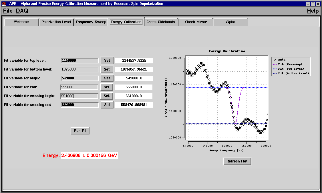
7. Energy Calibration
The fourth tab in APE's GUI window leads to the energy calibration.
The left side shows the fit parameters, a button to run the fit and as a result of this fit a read-back of the beam energy as well as its uncertainty. The right side shows a plot of I*tau vs sweep frequency. After a fit it will also show the fit curves for the upper and lower levels as well as the curve for the Froissart-Stora resonance crossing.
Procedure
Set the begin and end parameters (Hz of the sweep) which determine the fit interval. Then set top and the bottom level, which correspond to the I*tau before and after crossing the resonance. Finally set the beginning and end of the resonance crossing: The crossing begin is where the data starts to deviate from the top level whereas the crossing end is where the data starts to join the bottom level. See the picture as an example. Once all fit parameters are set, press the "Run Fit" button. The fit will first determine precise top and bottom levels. It will then calculate the resonance crossing according to Froissart-Stora and give back an updated energy value (from the central resonance frequency), its uncertainty (from the resonance width), update the fit parameters and show the calculated fit curves.
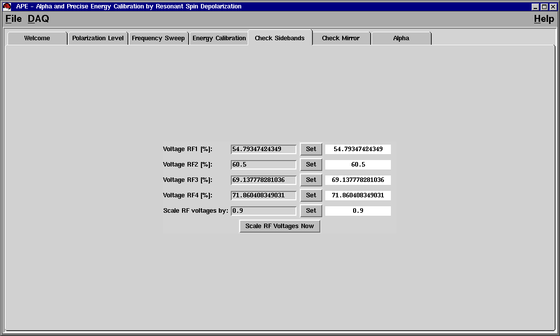
8. Check Sidebands
The fifth tab in APE's GUI window allows to check if the observed dip is the main resonance or one of its sidebands.
Procedure
The first four fields show the voltage on all four RF stations. Enter a factor by which the voltages should be scaled and press the button "Scale RF Voltages Now". Warning: Changing the RF voltages will change the synchrotron tune and thus perturb the beam! Only do this if you really know what you are doing. The RF voltages should be scaled simultaneously and you can now return to measure the resonance again.
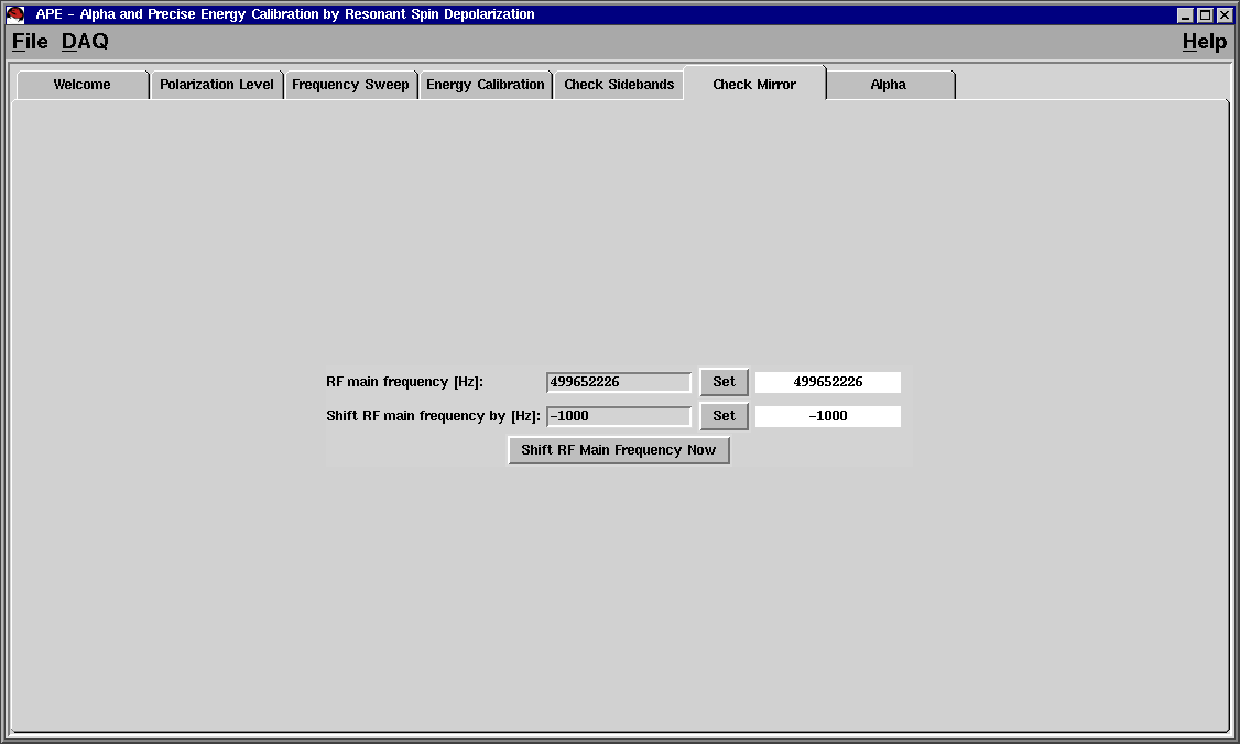
9. Check Mirror
The sixth tab in APE's GUI window allows to check if the observed dip is the main resonance or its mirror.
Procedure
The first field shows the RF main frequency. Enter a factor by which the frequency should be shifted and press the button "Shift RF Main Frequency Now". Warning: Changing the RF frequency will change the closed orbit and thus perturb the beam! Only do this if you really know what you are doing. Once the RF frequency is shifted you can return to measure the resonance again.
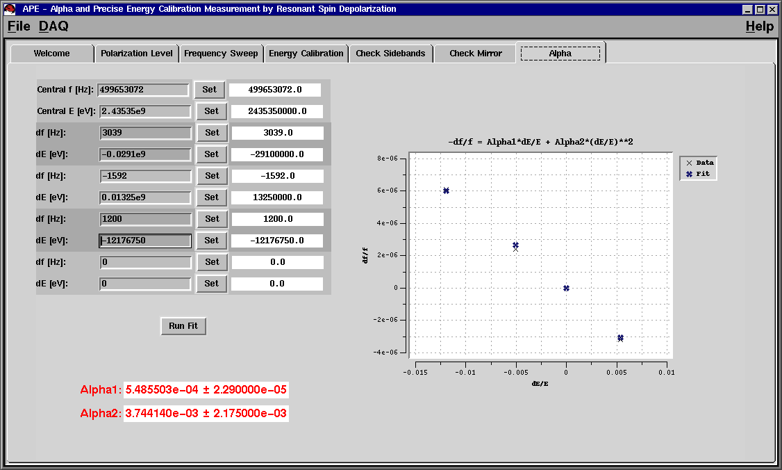
10. Alpha
The last tab in APE's GUI window allows to determine the momentum compaction factor Alpha to second order. The left side has entry fields for the data points; the right side shows the entered data points and the result of the alpha fit.
Procedure
Begin by entering the central RF frequency and the central energy of the unperturbed beam. Then enter AT LEAST two further pairs of data. The data pairs in the Alpha tab always consist of a the df (frequency shift) and the dE (resulting energy shift). Up to a maximum of four such data pairs can be entered. Enter zeros into the third and/or fourth data pair fields if you have measured less than four data points. Then press the "Run Fit" button to obtain values for the first and second order alpha coefficients. Three pairs of values (the central data pair and two additional data pairs) are required for the fit to be well-defined. More points render more precise alpha coefficients.
11. General Tips
APE will start even when a lock file is present if the user uses the ape.sh -f expression where -f is the force option. Still, make sure no other copies of APE are running and that there are no orphaned APE background processes running.
If you are unsure if APE is already done with a requested task, check APE's shell window. Normally a line will be written to show that a procedure has completed successfully.
If you need to read exact values from a plot (in order to set the fit start parameters for example), use the zoom function in the plot box. You can define a rectangle which shall be zoomed in on: Click once to set the upper left corner, click a second time to set the lower right corner; the zoom will follow immediately. To zoom back out again, do a single right-click. The cross-hairs can also help when reading values from data points in a plot.
If you have two sweeps with overlapping intervals, be sure to put their DAQs in separate files. If their DAQs are in the same file the plotted data for the energy calibration will show overlapping and will probably be a senseless mess due to the fact that a single sweep frequency will have several I*tau data points.